Covariance-based Structural Equation Modeling (CB-SEM)
Abstract
Structural equation modeling (SEM) is a versatile methodology widely applied in the social and behavioral sciences, epidemiology, economics, and other fields (Byrne, 2016; Schumacker & Lomax, 2010). SEM allows researchers to model causal relationships between unobservable latent variables (constructs such as attitudes) and observed variables (e.g., survey responses) using equations and path diagrams.
Covariance-based structural equation modeling (CB-SEM) is a statistical approach for estimating SEMs (Hair et al., 2018; Kline, 2023). CB-SEM relies on the covariance matrix of the observed data to test theoretical models and their fit. It assumes constructs are common factors and typically uses maximum likelihood (ML) estimation (Rigdon et al., 2017; Sarstedt et al., 2016).
As demonstrated in the tutorial article on CB-SEM in SmartPLS by Hair et al. (2025), SmartPLS supports graphical model building and CB-SEM estimation with ML. Results allow testing whether hypothesized model relationships are consistent with the data, positioning CB-SEM as a confirmatory, structure-testing procedure.
SmartPLS thus offers a modern alternative to other SEM software such as SPSS Amos.
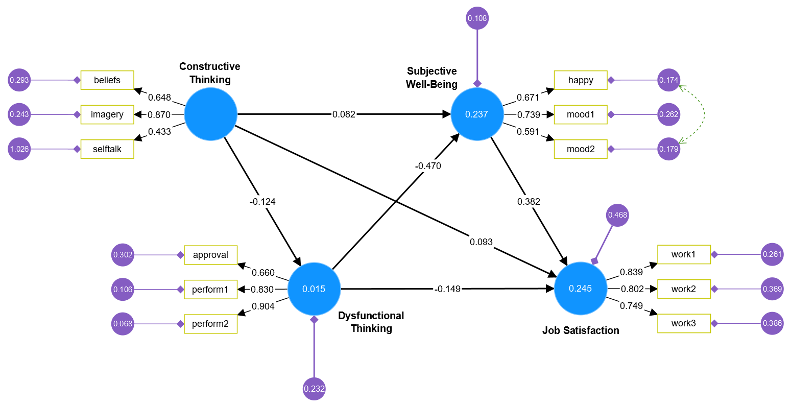
The following screenshot shows CB-SEM results in SmartPLS for Kline’s (2023) SEM textbook example on job satisfaction:

CB-SEM Algorithm Settings in SmartPLS
Maximum iterations
Specifies the maximum number of iterations the optimizer will perform. This should be set high enough to ensure convergence to a good solution.
- Default value: 1,000 (can be increased for complex models).
Starting value strategy
- Apply configured starting values
Use user-specified starting values defined in the theoretical model. If unchecked, default values are applied. - Default strategy
Mimics Lavaan’s default starting values:- Loading estimates: 1.0
- Path coefficients & covariances: 0.0
- Residual variances: 0.5 × indicator variance
- Latent variable variances: 0.05
- One-zero strategy
A simpler approach with:- Loadings: 1.0
- Variances: 1.0
- Path coefficients & covariances: 0.0
Stop criteria
- Gradient criterion
The optimizer stops when:||g|| < stop criterion × max(1, ||x||)- Default value: 10^-6
- Function value criterion
The optimizer stops when the improvement in the ML objective function is negligible:(f' – f) / f < stop criterion- Default value: 10^-9
Special assumptions
- Imply latent variable correlations
Estimates correlations between all exogenous latent variables, even if no correlation arrow is drawn. - Imply causal indicator correlations per construct
Estimates correlations between all causal indicators of a latent variable, even without correlation arrows. - Imply a variance of 1.0 for causal indicators
Constrains all causal indicator variances to 1.0, mimicking Lavaan’s defaults (overrides user-specified values).
Mean Structure
Most SEM analyses focus on modeling the covariance structure of observed variables. In special cases (e.g., latent growth curve modeling, multigroup analysis), including a mean structure may be necessary. A mean structure involves means and intercepts of latent and observed variables and requires constraints for identification (since only p observed means are available, with p = number of observed variables).
Options
- No mean structure (default)
Ignores means and estimates only covariances (sufficient for standard SEM). - Estimate mean structure, fix factor means to zero
Includes mean structure. Factor means are constrained to zero, observed variable intercepts are estimated freely. Additional constraints can be added by the user. - Estimate mean structure with only user-specified constraints
Includes mean structure without predefined constraints. The user must specify all necessary identification constraints.
CB-SEM Examples in SmartPLS
SmartPLS provides directly computable CB-SEM examples from leading textbooks (Byrne, 2016; Hair et al., 2018; Kline, 2023; Schumacker & Lomax, 2010). The results in SmartPLS replicate the textbook examples exactly. Try out the CB-SEM example projects in SmartPLS
References
- Byrne, B. M. (2016). Structural Equation Modeling with AMOS: Basic Concepts, Applications, and Programming (Multivariate Applications) (3 ed.). Routledge.
- Hair, J. F., Babin, B. J. Ringle, C. M., Sarstedt, M., & Becker, J.-M. (2025): Covariance-based Structural Equation Modeling (CB-SEM): A SmartPLS 4 Software Tutorial. Journal of Marketing Analytics, forthcoming.
- Hair, J. F., Black, W. C., Babin, B. J., & Anderson, R. E. (2018). Multivariate Data Analysis (8 ed.). Cengage Learning.
- Kline, R. B. (2023). Principles and Practice of Structural Equation Modeling (5 ed.). Guilford Press.
- Schumacker, R. E., & Lomax, R. G. (2010). A Beginner's Guide to Structural Equation Modeling (3 ed.). Routledge.
- Rigdon, E. E., Sarstedt, M. & Ringle, C. M. (2017). On Comparing Results from CB-SEM and PLS-SEM. Five Perspectives and Five Recommendations. Marketing ZFP, 39(3), 4-16.
- Sarstedt, M., Hair, J. F. Ringle, C. M., Thiele, K. O., & Gudergan, S.P. (2016). Estimation Issues with PLS and CBSEM: Where the Bias Lies!, Journal of Business Research, 69 (2016), Issue 10, pp. 3998-4010.
- More literature ...
Cite correctly
Please always cite the use of SmartPLS!
Ringle, Christian M., Wende, Sven, & Becker, Jan-Michael. (2024). SmartPLS 4. Bönningstedt: SmartPLS. Retrieved from https://www.smartpls.com

