Moderator Analysis in CB-SEM
Moderator analysis in covariance-based structural equation modeling (CB-SEM) examines whether the strength or direction of a structural relationship between two latent constructs depends on the level of a third construct, the moderator. This allows researchers to test conditional relationships and uncover more nuanced insights than a single, constant effect would show. Unlike PLS-SEM, where product-indicator and two-stage approaches are common, CB-SEM focuses on latent interaction modeling within the covariance structure. Currently, SmartPLS only supports two-way interactions for CB-SEM moderation.
How Moderation Works in CB-SEM
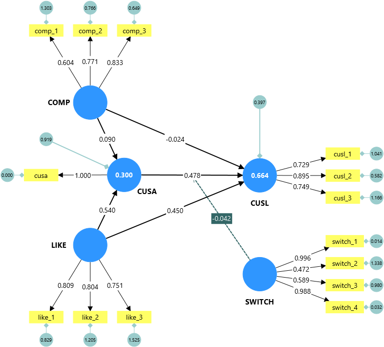
A moderator variable affects the relationship between an independent variable (predictor) and a dependent variable (outcome). The presence of moderation implies that the predictor’s effect is not constant but varies depending on the moderator. In the example shown in the figure:
- CUSA → CUSL is the simple effect.
- SWITCH is introduced as a moderator.
- The moderation path is drawn from SWITCH to the CUSA → CUSL relationship, which creates the interaction construct (CUSA × SWITCH).
- The interaction construct is then linked to CUSL.
- A negative coefficient (e.g., –0.042) suggests that higher SWITCH values weaken the positive effect of CUSA on CUSL.
- Bootstrapping can be applied to test whether this effect is statistically significant.
- The Simple Slope Plot provides an intuitive visualization of this moderating effect.
Creating Moderation in CB-SEM
In SmartPLS, when using CB-SEM models, moderation is set up as follows:
- Define the constructs: Independent (predictor), dependent (outcome), and moderator.
- Draw the moderation path: In SmartPLS, moderation is implemented by drawing a path from the moderator construct onto the existing path between the independent and dependent construct. This step tells the software that the moderator should influence the strength of that specific relationship.
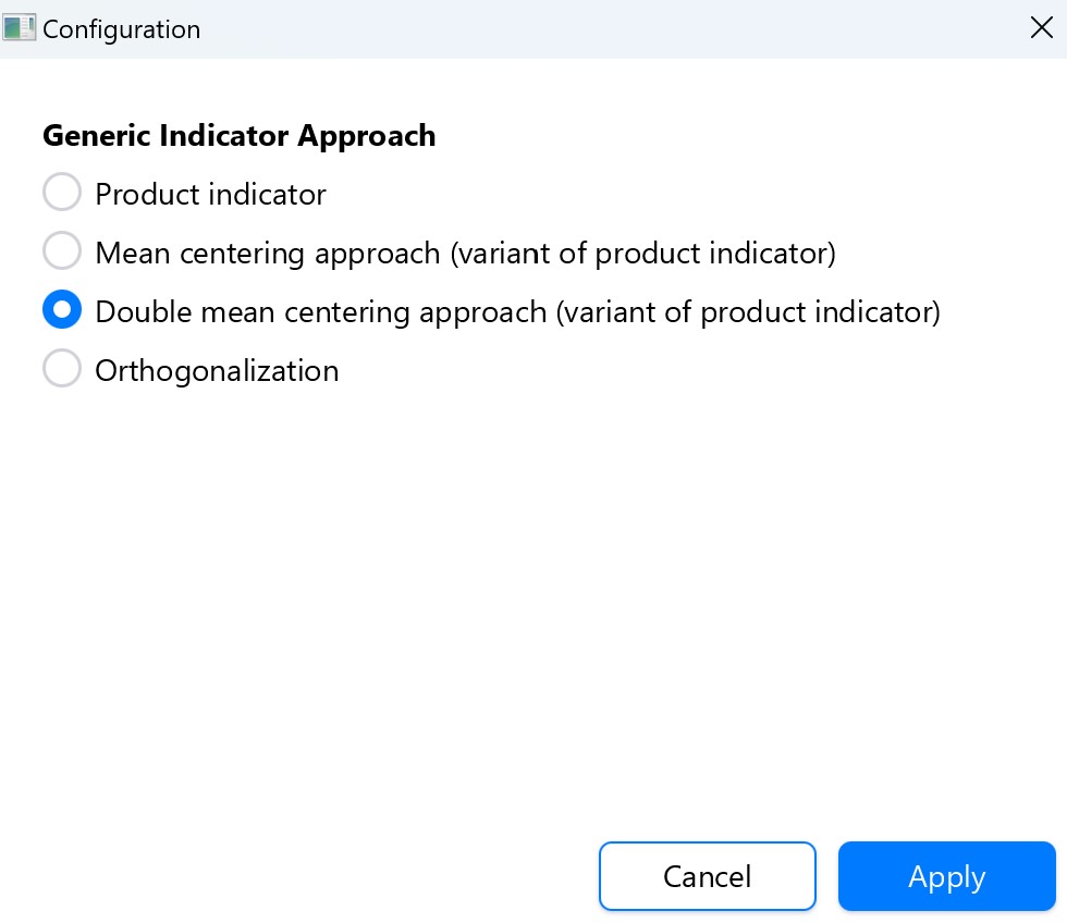
- Interaction computation dialog: Once you double-click the moderation path, SmartPLS opens a dialog to choose how the interaction term should be computed.
- Add the interaction path: The software generates an interaction construct (predictor × moderator) and links it to the dependent construct.
- Estimate the model: Run the CB-SEM algorithm to obtain the standardized path coefficients.
- The Bootstrapping procedure can be used to assess the significance of the moderation effect.
Approaches to Compute the Interaction Term
After double-clicking on the interaction path of the SmartPLS moderator analysis model a dialog opens which offers several computation approaches for the interaction term:
| Approach | Description |
|---|---|
| Generic indicator approach | Uses all available product terms between the predictor and moderator indicators. Straightforward but can add many indicators (higher model complexity). |
| Product indicator approach | Multiplies each predictor indicator with each moderator indicator. Classic, widely used baseline. |
| Mean centering approach (variant of product indicator) | Mean-centers indicators before forming products to reduce multicollinearity between main effects and the interaction. |
| Double mean centering approach (variant of product indicator, default) | Mean-centers each indicator and also subtracts the product of the indicator means. Provides stronger reduction in collinearity and is the default option in SmartPLS CB-SEM. |
| Orthogonalization | Forms product terms and then removes variance explained by the main effects. Ensures the interaction is uncorrelated with them, reducing collinearity even more effectively. |
Inspecting Simple Slope Plots
In the results report, researchers can further analyze moderation effects by inspecting the Simple Slope Plot. This plot visualizes how the effect of the predictor on the dependent variable changes at different levels of the moderator (e.g., low, mean, high).
In this example:
- The red line shows the effect of CUSA on CUSL when SWITCH is one standard deviation below the mean.
- The blue line shows the effect at the mean level of SWITCH.
- The green line shows the effect when SWITCH is one standard deviation above the mean.
This visualization helps researchers interpret whether the moderation strengthens or weakens the predictor–outcome relationship at different moderator levels.
CB-SEM Examples in SmartPLS
SmartPLS provides directly computable CB-SEM moderator analysis and multigroup analysis examples from leading textbooks (Hair et al., 2018; Hair et al., 2022). Try out the CB-SEM example projects in SmartPLS. Alternatively, you can run a CB-SEM multigroup (MGA) analysis.
Frequently Asked Questions
How does CB-SEM handle moderation differently from PLS-SEM?
PLS-SEM commonly relies on product-indicator or two-stage approaches to model moderation. CB-SEM instead uses latent interaction modeling within the covariance structure. SmartPLS currently supports two-way interactions for CB-SEM moderation.
How do I set up a moderator effect in SmartPLS CB-SEM models?
Define the independent (predictor), dependent (outcome), and moderator constructs, then draw the moderation path from the moderator construct onto the existing path between the independent and dependent construct. SmartPLS then opens a dialog to choose how the interaction term should be computed, generates the interaction construct, and links it to the dependent construct so the model can be estimated.
Which interaction term computation approach is the default in SmartPLS?
The double mean centering approach is the default. It mean-centers each indicator and also subtracts the product of the indicator means, which provides a stronger reduction in collinearity than the plain product indicator or single mean centering approaches.
How can I test whether a moderation effect is statistically significant?
After estimating the model, use the bootstrapping procedure to assess whether the standardized path coefficient of the interaction term is statistically significant.
What does the Simple Slope Plot show?
The Simple Slope Plot visualizes how the effect of the predictor on the dependent variable changes at different levels of the moderator, typically shown as separate lines for one standard deviation below the mean, at the mean, and one standard deviation above the mean. This helps researchers see whether the moderation strengthens or weakens the predictor-outcome relationship.
Related SmartPLS Methods
References
- Hair, J. F., Black, W. C., Babin, B. J., & Anderson, R. E. (2018). Multivariate data analysis (8th ed.). Cengage Learning.
- Hair, J. F., Hult, G. T. M., Ringle, C. M., & Sarstedt, M. (2027). A primer on partial least squares structural equation modeling (PLS-SEM) (4th ed.). Sage.
- More literature ...
Cite correctly
Please always cite the use of SmartPLS!
Ringle, Christian M., Wende, Sven, & Becker, Jan-Michael. (2024). SmartPLS 4. Bönningstedt: SmartPLS. Retrieved from https://www.smartpls.com
