
Logistic Regression
Logistic regression explains and predicts a binary (dichotomous) dependent variable, such as 0/1, yes/no, purchase/no purchase, or churn/no churn, from one or more independent variables. Unlike linear regression, logistic regression models the probability of belonging to one of the two outcome categories and therefore keeps predicted probabilities between 0 and 1.
SmartPLS (Ringle et al., 2024) estimates logistic regression models by maximum likelihood and provides a comprehensive results report with regression coefficients, significance tests, odds ratios, model-fit measures, predicted probabilities, classification results, a cutoff chart, and receiver operating characteristic (ROC) analysis. A detailed SmartPLS tutorial for multiple linear and logistic regression is provided by Margalina et al. (2026), using the HBAT example from Hair et al. (2019).
When to Use Logistic Regression
Use logistic regression when the dependent variable has exactly two categories. Examples include whether a customer churns (
0 = no, 1 = yes), whether an applicant defaults (0 = no, 1 = yes), or whether a customer belongs to one of two market segments.The independent variables can be metric or categorical. Categorical predictors with more than two categories must be represented by appropriate contrasts, such as dummy variables, before they enter the regression model. As with all regression analyses, predictor selection should be theoretically justified and the model should contain the variables required to address the research question (Hair et al., 2019; Margalina et al., 2026).
Understanding Logistic Regression
Logistic regression predicts the probability of the focal outcome, usually coded as
Y = 1. If p denotes the probability that Y = 1, the odds are:Odds = p / (1 - p)The natural logarithm of the odds is the logit:
logit(p) = ln[p / (1 - p)] = beta0 + beta1*X1 + ... + betap*XpThe logit can be transformed back into a probability between 0 and 1:
p = exp(logit) / [1 + exp(logit)]This transformation is the key difference from linear regression. A logistic regression coefficient therefore represents the expected change in the log-odds of
Y = 1 for a one-unit increase in the predictor, holding all other predictors constant. It is not a direct change in probability.For easier interpretation, SmartPLS also reports the exponentiated coefficient,
Exp(Coefficients), which is the odds ratio:Exp(beta) = 1: the odds do not change.Exp(beta) > 1: the odds ofY = 1increase.Exp(beta) < 1: the odds ofY = 1decrease.
For example, an odds ratio of 1.50 means that a one-unit increase in the predictor multiplies the odds of the focal outcome by 1.50, corresponding to a 50% increase in the odds. An odds ratio of 0.80 corresponds to a 20% decrease in the odds.
Logistic Regression in SmartPLS: HBAT Example
The SmartPLS logistic regression example follows the HBAT case used by Hair et al. (2019, Chap. 8) and Margalina et al. (2026). The dependent variable is Region (X4), coded
0 = USA/North America and 1 = outside North America. The independent variables X6 to X18 capture customers' perceptions of HBAT's performance, including product quality, e-commerce activities, technical support, complaint resolution, advertising, product line, salesforce image, competitive pricing, warranty and claims, new products, ordering and billing, price flexibility, and delivery speed.The graphical output shows the estimated logistic regression coefficients for all predictors and the intercept. The value displayed inside the dependent variable X4 (
0.643) corresponds to Cox and Snell's pseudo R-square for this model.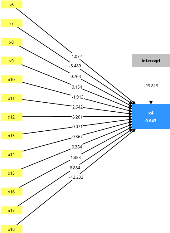
Figure 1. Logistic regression model results for the HBAT example in SmartPLS.
The model is estimated using all 100 observations in the HBAT dataset. As emphasized by Margalina et al. (2026), this sample is small relative to the number of predictors and is primarily suitable as an instructional example. Predictive claims should therefore be supported by holdout-sample or other out-of-sample validation.
Logistic Regression Settings in SmartPLS
Select Calculate > Logistic Regression to estimate the model. SmartPLS provides the following settings:
| Setting | What it controls |
|---|---|
| Test type | Specifies whether a one-sided or two-sided significance test is conducted. |
| Significance level | Specifies the significance level used for the coefficient tests. |
| Maximum iterations | Specifies the maximum number of maximum-likelihood iterations. This prevents the algorithm from running indefinitely if the model does not converge. Increasing this value can help when convergence requires additional iterations, but nonconvergence should always be investigated. |
| Stop criterion | Specifies the convergence criterion. The algorithm terminates when the change in log-likelihood between two consecutive iterations falls below this threshold or when the maximum number of iterations is reached. |
SmartPLS uses maximum likelihood estimation with Newton-Raphson iterations for logistic regression. In the HBAT example, the algorithm converges after 8 iterations, with a final log-likelihood difference of approximately
6.52e-8, which is below the selected stopping criterion of 10^-5.When an intercept is included in the graphical regression model, SmartPLS estimates the intercept. To estimate a logistic regression model without an intercept, select the intercept in the model and delete it before running the analysis.
Evaluating Logistic Regression Results
A logistic regression model should not be evaluated using a single statistic. The assessment should cover algorithm convergence, overall model fit, coefficient significance and direction, odds ratios, predicted probabilities, classification performance, the classification cutoff, and threshold-independent discrimination using ROC analysis (Hair et al., 2019; Margalina et al., 2026).
1. Check Algorithm Convergence
Before interpreting the results, verify that the maximum-likelihood algorithm converged. In Algorithm > Estimation summary, SmartPLS reports the number of iterations used and the final log-likelihood difference.
If the maximum number of iterations is reached before the stopping criterion is satisfied, the estimates should not be interpreted without investigating the source of nonconvergence. Potential causes include an overly complex model relative to the sample size, highly correlated predictors, or data patterns that make coefficient estimation unstable.
2. Assess Overall Model Fit
Open Model fit > Fit summary. SmartPLS reports the log-likelihood, deviance, Akaike information criterion (AIC), Bayesian information criterion (BIC), and three pseudo R-square measures.
For the HBAT example, the estimated model produces the following results:
| Measure | Null model | Estimated model |
|---|---|---|
| LogLikelihood | -66.875 | -15.394 |
| Deviance (-2LL) | 133.750 | 30.789 |
| AIC | 135.750 | 58.789 |
| BIC | 138.355 | 95.261 |
| Cox and Snell's R-square | — | 0.643 |
| Nagelkerke's R-square | — | 0.872 |
| McFadden's R-square | — | 0.770 |
The substantially lower deviance of the estimated model relative to the null model indicates a strong improvement in fit. Lower AIC and BIC values likewise favor the estimated model when comparing models for the same dependent variable and dataset. AIC and BIC are relative model-comparison criteria; they should not be interpreted as absolute goodness-of-fit thresholds.
The pseudo R-square measures summarize improvement in model fit from different likelihood-based perspectives. They are useful for describing and comparing logistic regression models, but they are not equivalent to the R-square in ordinary least squares regression and should not be interpreted as the percentage of variance explained in the same way (Hair et al., 2019; Margalina et al., 2026).
3. Interpret Coefficients, Wald Tests, and Odds Ratios
Open Final results > Coefficients. SmartPLS reports:
- Coefficients: estimated effects on the log-odds of
Y = 1. - SE: standard errors of the coefficient estimates.
- z-statistic: coefficient divided by its standard error.
- Wald: Wald statistic for testing whether a coefficient equals zero.
- P value: significance level of the coefficient test.
- Exp(Coefficients): exponentiated coefficient, or odds ratio.
In the HBAT example, three predictors are statistically significant at the 5% level:
| Predictor | Coefficient | P value | Odds ratio |
|---|---|---|---|
| X7 E-Commerce Activities/Website | -5.489 | 0.016 | 0.004 |
| X10 Advertising | -1.912 | 0.033 | 0.148 |
| X12 Salesforce Image | 8.201 | 0.008 | 3645.181 |
The negative coefficients for X7 and X10 indicate that higher values are associated with lower odds of belonging to the
X4 = 1 group, holding the other predictors constant. The positive coefficient for X12 indicates higher odds of belonging to the X4 = 1 group.Odds ratios are often easier to communicate than log-odds. For example, the odds ratio of 0.148 for X10 means that a one-unit increase in advertising perception multiplies the odds of
X4 = 1 by 0.148, corresponding to an approximately 85.2% reduction in the odds. Very large or very small odds ratios, such as those in this small HBAT example, should be interpreted cautiously and together with the standard errors, sample size, model specification, and validation results.4. Examine Predicted Probabilities and the Confusion Matrix
Under Final results > Predictions and probabilities, SmartPLS reports the predicted probability
P(Y = 1 | X) for every observation and the corresponding predicted class.The confusion matrix compares the observed and predicted classes. For the HBAT example, the result is:
| Observed class | Predicted 0 | Predicted 1 | Percentage correct |
|---|---|---|---|
| X4 = 0 | 38 | 1 | 97.436% |
| X4 = 1 | 5 | 56 | 91.803% |
Thus, 38 of the 39 observations from class 0 and 56 of the 61 observations from class 1 are classified correctly under the cutoff used for the reported classification results.
5. Evaluate Accuracy, Sensitivity, Specificity, Precision, and AUC
SmartPLS reports several complementary classification measures:
| Measure | HBAT result | Interpretation |
|---|---|---|
| Accuracy | 0.940 | Share of all observations classified correctly. |
| Sensitivity / Recall | 0.918 | Share of actual positive cases (Y = 1) classified as positive. |
| Specificity | 0.974 | Share of actual negative cases (Y = 0) classified as negative. |
| Precision | 0.982 | Share of predicted positive cases that are actually positive. |
| AUC | 0.983 | Threshold-independent measure of discrimination between the two classes. |
These measures answer different questions. Accuracy summarizes overall classification success, sensitivity focuses on correctly identifying positive cases, specificity focuses on correctly identifying negative cases, and precision focuses on the reliability of positive predictions. Which measure deserves the greatest emphasis depends on the substantive consequences of false positives and false negatives.
6. Use the Cutoff Chart to Select and Evaluate Classification Thresholds
Predicted probabilities must be converted into class predictions using a cutoff, also called a classification threshold. Observations with predicted probabilities above the cutoff are assigned to the focal class (
Y = 1), whereas observations below the cutoff are assigned to the other class (Y = 0).The choice of cutoff affects classification performance. A lower cutoff generally classifies more observations as positive, which tends to increase sensitivity but reduce specificity. A higher cutoff generally classifies fewer observations as positive, which tends to increase specificity but reduce sensitivity. Precision and overall accuracy can also change substantially.
SmartPLS therefore provides a cutoff chart that shows how accuracy, sensitivity/recall, specificity, and precision change across classification thresholds.
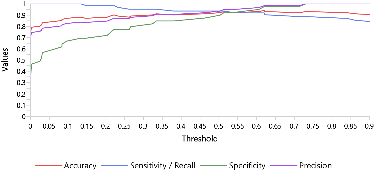
Figure 2. Cutoff chart for the HBAT logistic regression example in SmartPLS.
The chart should not be used to select a cutoff mechanically. The appropriate threshold depends on the purpose of the analysis, the relative costs of false positives and false negatives, and the prevalence of the two outcome classes. When the cutoff is selected using the same data used to estimate the model, the resulting performance remains in-sample. For predictive applications, the model and the selected cutoff should be evaluated on a holdout sample or by another suitable out-of-sample validation procedure (Hair et al., 2019).
7. Evaluate the ROC Curve and AUC
The receiver operating characteristic (ROC) curve evaluates the model's ability to discriminate between the two outcome classes across all possible classification thresholds. A standard ROC curve plots the false positive rate (
1 - specificity) on the x-axis and the true positive rate (sensitivity/recall) on the y-axis. Each point represents a different cutoff. The diagonal reference line represents discrimination no better than random classification.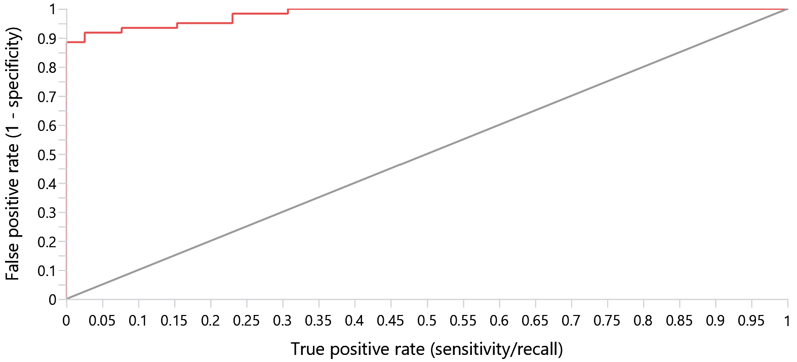
Figure 3. ROC curve for the HBAT logistic regression example in SmartPLS.
SmartPLS additionally reports the area under the ROC curve (AUC). An AUC of 0.50 indicates no discrimination beyond random ranking, whereas an AUC of 1.00 indicates perfect discrimination. The HBAT model yields an AUC of 0.983, indicating excellent in-sample discrimination between the two regional groups.
The ROC curve and AUC complement the cutoff chart. The cutoff chart is threshold-dependent and helps evaluate the consequences of choosing a particular cutoff. AUC is threshold-independent and summarizes discrimination across the full range of cutoffs. A high AUC does not, however, establish that predicted probabilities are perfectly calibrated or that the model will achieve the same performance in new data.
The addition of ROC analysis extends the SmartPLS logistic regression output beyond the functionality documented by Margalina et al. (2026), who identified ROC analysis as an important extension for assessing predictive accuracy more comprehensively.
Logistic Regression Assumptions and Validation
Logistic regression does not require normally distributed residuals or homoscedasticity in the same way as ordinary least squares regression. Important considerations include (Hair et al., 2019; Margalina et al., 2026):
- Binary dependent variable: the outcome must have two categories.
- Independent observations: observations should not violate the independence assumptions implied by the research design.
- No perfect multicollinearity: predictors should not be exact linear combinations of one another, and problematic collinearity should be avoided.
- Linearity in the logit: continuous predictors should relate approximately linearly to the log-odds, not necessarily to the outcome probability itself.
- Adequate sample information: maximum likelihood estimation requires sufficient observations and sufficient information in both outcome categories to obtain stable estimates.
- Validation for predictive claims: classification accuracy, cutoff performance, and AUC should be evaluated on new data when the goal is prediction.
The HBAT example contains 100 observations and 13 predictors. Its very high accuracy and AUC are therefore best treated as illustrative in-sample results, not as evidence that the model will achieve the same predictive performance in another sample.
Recommended Workflow for Logistic Regression in SmartPLS
A practical workflow is:
- Define the binary dependent variable and identify which category is coded as
1. - Specify theoretically justified independent variables and the intercept, if required.
- Run Calculate > Logistic Regression and verify algorithm convergence.
- Assess the fit summary, including log-likelihood, deviance, AIC, BIC, and pseudo R-square measures.
- Interpret coefficients, Wald tests, p values, and odds ratios.
- Inspect predicted probabilities and the confusion matrix.
- Evaluate accuracy, sensitivity/recall, specificity, and precision.
- Use the cutoff chart to understand the consequences of alternative classification thresholds.
- Evaluate the ROC curve and AUC for threshold-independent discrimination.
- Validate predictive performance using a holdout sample or another out-of-sample procedure when prediction is an objective.
This workflow follows the general regression assessment logic described by Hair et al. (2019) and the SmartPLS-specific guidance provided by Margalina et al. (2026).
Frequently Asked Questions
When should I use logistic regression instead of linear regression?
Use logistic regression when the dependent variable is dichotomous. Linear regression is designed for a continuous metric dependent variable and can produce predicted values below 0 or above 1 when applied to binary outcomes. Logistic regression models the probability of the focal category within the admissible 0-to-1 range.
How does SmartPLS estimate logistic regression models?
SmartPLS estimates logistic regression coefficients by maximum likelihood using Newton-Raphson iterations. The results include coefficients, standard errors, Wald tests, p values, odds ratios, predicted probabilities, classification metrics, model-fit measures, cutoff analysis, ROC curves, and AUC.
What does a logistic regression coefficient mean?
A coefficient represents the change in the log-odds of the focal outcome (
Y = 1) for a one-unit increase in the predictor while holding the other predictors constant. It is not a direct change in probability.What does Exp(Coefficients) mean in SmartPLS?
Exp(Coefficients) is the odds ratio. Values above 1 indicate increasing odds of Y = 1, values below 1 indicate decreasing odds, and a value of 1 indicates no change in the odds.What is the difference between the cutoff chart and the ROC curve?
The cutoff chart shows how classification measures such as accuracy, sensitivity, specificity, and precision change when the probability threshold changes. The ROC curve evaluates the trade-off between sensitivity and the false positive rate across all thresholds. AUC summarizes the ROC curve in one threshold-independent discrimination statistic.
What is a good cutoff for logistic regression?
There is no universally best cutoff. The appropriate threshold depends on the decision context, the relative costs of false positives and false negatives, and the class distribution. When prediction is the objective, a cutoff selected on the estimation sample should be validated on new data.
Is pseudo R-square the same as R-square in linear regression?
No. Cox and Snell's, Nagelkerke's, and McFadden's pseudo R-square measures are likelihood-based measures of model fit. They should not be interpreted as the percentage of variance explained in the same way as the R-square from ordinary least squares regression.
Does a high AUC mean that predicted probabilities are accurate?
Not necessarily. AUC measures discrimination, meaning how well the model separates or ranks observations from the two outcome classes. It does not by itself establish probability calibration or out-of-sample predictive performance.
How do I estimate a logistic regression model without an intercept?
If an intercept is included in the graphical model, SmartPLS estimates it. To exclude the intercept, select it in the graphical model specification and delete it before running the logistic regression analysis.
What do the maximum iterations and stop criterion settings do?
Maximum iterations limits the number of maximum-likelihood iterations. The stop criterion specifies how small the change in log-likelihood must become before SmartPLS treats the estimation as converged. If the algorithm reaches the maximum number of iterations without satisfying the stop criterion, investigate the model and data before interpreting the estimates.
Related SmartPLS Methods
References
- Backhaus, K., Erichson, B., Gensler, S., Weiber, R., & Weiber, T. (2021). Multivariate analysis: An application-oriented introduction. Springer.
- Hair, J. F., Black, W. C., Babin, B. J., & Anderson, R. E. (2019). Multivariate data analysis (8th ed.). Cengage Learning.
- Hanley, J. A., & McNeil, B. J. (1982). The meaning and use of the area under a receiver operating characteristic (ROC) curve. Radiology, 143(1), 29-36. https://doi.org/10.1148/radiology.143.1.7063747
- Margalina, V.-M., Kreienbaum, C., Hair, J. F., Becker, J.-M., & Ringle, C. M. (2026). Multiple linear and logistic regression analysis: A SmartPLS 4 software tutorial. Journal of Marketing Analytics, 14, 709-726. https://doi.org/10.1057/s41270-026-00466-2
- Ringle, C. M., Wende, S., & Becker, J.-M. (2024). SmartPLS 4. In SmartPLS. https://www.smartpls.com/
Cite correctly
Please always cite the use of SmartPLS!
Ringle, Christian M., Wende, Sven, & Becker, Jan-Michael. (2024). SmartPLS 4. Bönningstedt: SmartPLS. Retrieved from https://www.smartpls.com
