
On this page
Linear Regression Analysis in SmartPLS
Linear regression explains or predicts the value of a single dependent (criterion or outcome) variable from one or more independent (predictor or explanatory) variables. A model with one predictor is a simple linear regression; a model with two or more predictors is a multiple linear regression. SmartPLS (Ringle et al., 2024) lets you specify and estimate both types of regression models graphically and provides a comprehensive results report with coefficients, model evaluation criteria, collinearity statistics, residual diagnostics, predicted values, and integrated importance-performance map analysis (IPMA) results. For a comprehensive step-by-step tutorial on multiple linear and logistic regression analysis in SmartPLS, including model specification, estimation, assumption assessment, and result interpretation, see Margalina et al. (2026).
What Linear Regression Does
As described by Hair, Black, Babin, and Anderson (2018), multiple regression analysis examines the relationship between one dependent variable and several independent variables (see also Backhaus, Erichson, Gensler, Weiber, & Weiber, 2021; Sarstedt & Mooi, 2019). Margalina et al. (2026) provide a SmartPLS-focused treatment of these principles and emphasize the three central purposes of regression analysis: testing relationships, assessing the relative contribution of predictors, and making predictions. The estimated regression equation combines the independent variables so that their weighted values predict the dependent variable.
Each regression coefficient represents the estimated relationship between an independent variable and the dependent variable while holding the other predictors in the model constant. SmartPLS reports both unstandardized coefficients, which retain the variables' original units, and standardized coefficients, which facilitate comparisons of relative effect magnitudes across predictors. When predictors are strongly correlated, however, coefficient estimates can become unstable and their individual interpretation becomes more difficult. Researchers should therefore evaluate collinearity diagnostics together with the coefficients.
Linear regression can support both explanatory and predictive research objectives. However, a regression coefficient by itself does not establish a causal relationship; causal interpretation requires an appropriate research design and identification strategy.
Regression Models and Result Reports in SmartPLS
The following figure illustrates a multiple regression model specified in SmartPLS. When an intercept is included in the graphical model, SmartPLS estimates it together with the regression coefficients. To estimate a regression model without an intercept, select and delete the intercept from the graphical model specification.

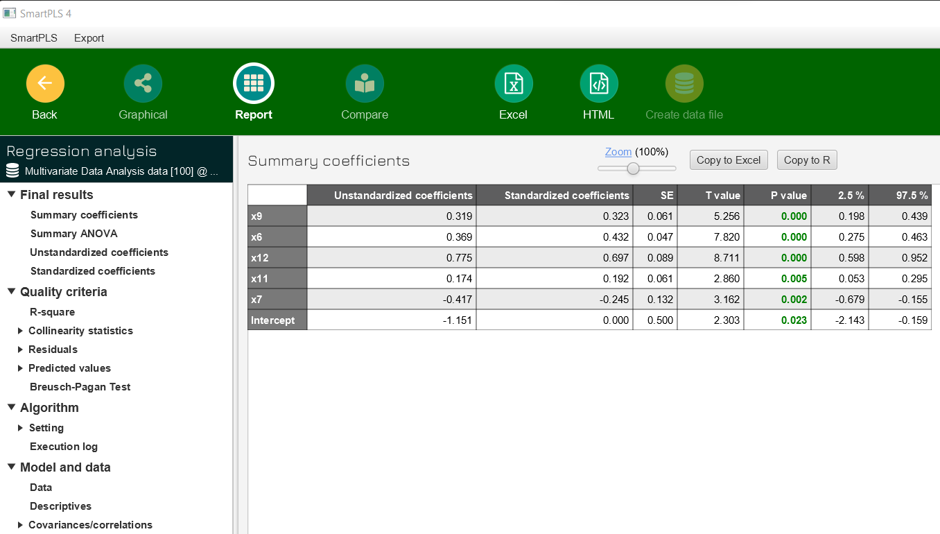
The regression results report provides the information needed for a systematic model evaluation. Depending on the model and settings, the report includes summary coefficients, ANOVA results, unstandardized and standardized coefficients, R-square results, collinearity statistics, residual diagnostics, predicted values, the Breusch-Pagan test, descriptive statistics, and covariance/correlation information. Margalina et al. (2026) demonstrate how these results can be evaluated in a structured workflow in SmartPLS.
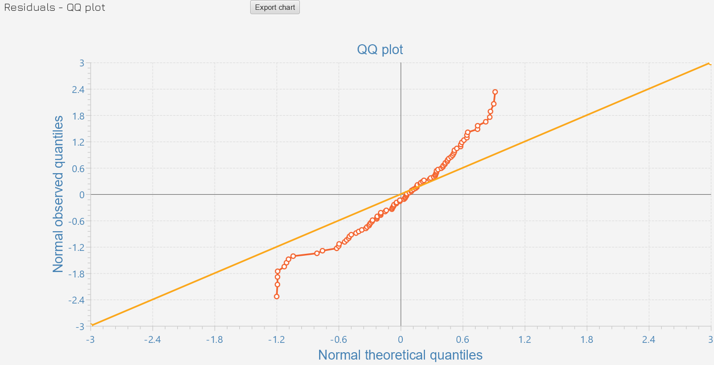
SmartPLS also provides graphical regression diagnostics. For example, the residual QQ plot compares the observed residual quantiles with the theoretical quantiles of a normal distribution. Systematic departures from the reference line indicate departures from residual normality.
How to Evaluate Linear Regression Results in SmartPLS
A systematic evaluation should consider several complementary aspects rather than focusing only on p values. The sequence below reflects the regression evaluation logic and SmartPLS workflow illustrated by Margalina et al. (2026).
1. Regression Coefficients and Statistical Inference
Inspect the unstandardized and standardized coefficients, standard errors, t values, p values, and confidence intervals. The sign of a coefficient indicates the direction of the estimated relationship, while its magnitude indicates the strength of that relationship conditional on the other predictors in the model. Unstandardized coefficients express the expected change in the dependent variable for a one-unit change in a predictor, whereas standardized coefficients facilitate comparisons of relative importance across predictors measured on different scales (Margalina et al., 2026).
For nonparametric inference based on resampling, SmartPLS also offers regression bootstrapping.
2. Explained Variance and Overall Model Results
Use R-square (R²) to assess the proportion of variance in the dependent variable explained by the predictors. Adjusted R-square accounts for model complexity and is especially useful when comparing regression models with different numbers of predictors. The ANOVA results provide an omnibus assessment of whether the regression model with its predictors improves on an intercept-only model. Margalina et al. (2026) illustrate the joint interpretation of ANOVA, R², and adjusted R² in the SmartPLS regression results report.
3. Collinearity
Inspect the collinearity statistics before interpreting individual regression coefficients. High collinearity among predictors can inflate standard errors, destabilize coefficients, and make it difficult to distinguish the predictors' separate contributions. SmartPLS reports the variance inflation factor (VIF) and the condition index as complementary collinearity diagnostics; Margalina et al. (2026) demonstrate their use before interpreting the regression coefficients.
4. Residual Diagnostics and Heteroscedasticity
Use the residual results and plots to inspect the regression assumptions. SmartPLS provides several complementary diagnostics, including predicted-versus-residual plots for detecting nonlinear patterns and heteroscedasticity, predicted-versus-actual plots for inspecting the fitted relationship, a residual autocorrelation plot and the Durbin-Watson test for residual independence, and a QQ plot and residual histogram for evaluating residual normality. The Breusch-Pagan test formally assesses homoscedasticity; a statistically significant result indicates evidence of heteroscedasticity. Margalina et al. (2026) provide a worked SmartPLS example of these diagnostics. When heteroscedasticity is a concern, consider the HC3 or HC4 standard error options described below.
5. Predicted Values
The predicted-values section helps researchers inspect the model's fitted outcomes and individual prediction errors. These in-sample results should not be confused with out-of-sample predictive assessment.
6. Importance-Performance Map Analysis (IPMA)
SmartPLS integrates importance-performance map analysis (IPMA) directly into the results of every linear regression analysis. For regression models, IPMA is not executed as a separate algorithm. Instead, the IPMA results are available within the standard linear regression results report. This extends the regression analysis beyond conventional significance and coefficient assessment by combining the predictors' importance with their performance; Margalina et al. (2026) specifically highlight IPMA as a complementary analysis for gaining additional insight from SmartPLS regression results (see also Ringle & Sarstedt, 2016).
IPMA complements the usual coefficient-based interpretation by considering two dimensions simultaneously:
- Importance: the estimated effect of an independent variable on the dependent target variable.
- Performance: the current level of the independent variable, represented on a common performance scale.
This combination is particularly useful for prioritization. When importance values are positive, independent variables with relatively high importance but comparatively low performance are potential priorities for improvement because changes in these variables may offer greater leverage for improving the target outcome. Negative importance values require the opposite directional interpretation and should not be treated as improvement priorities in the same way.
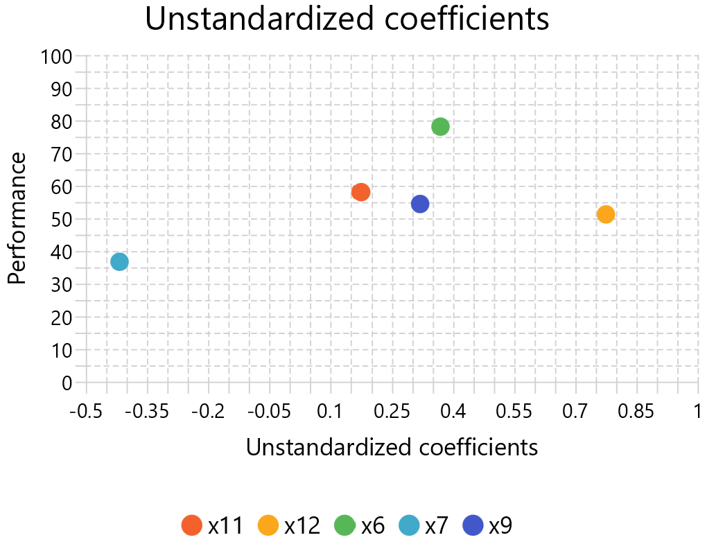
The following importance-performance map illustrates the regression IPMA results based on unstandardized coefficients. The horizontal axis shows the unstandardized regression coefficients, which represent the predictors’ importance for the dependent variable, while the vertical axis shows their performance on the 0-to-100 scale. Each point represents one independent variable. Predictors farther to the right have greater positive importance; among predictors with similar importance, those with lower performance indicate comparatively greater potential for improvement. Predictors with negative coefficients require a directionally reversed interpretation.
The conceptual logic follows the IPMA used in PLS-SEM. For background on importance and performance, interpretation of importance-performance maps, and the role of variable ranges, see the Importance-Performance Map Analysis (IPMA) documentation for PLS-SEM. In particular, verify the theoretically possible minimum and maximum values of the variables used to calculate performance scores; incorrect scale ranges can distort the 0-to-100 performance transformation.
Important distinction: In PLS-SEM, IPMA is available as a dedicated analysis with a selected target construct. In linear regression, SmartPLS provides IPMA results automatically as part of the regression results report, with the regression's dependent variable serving as the target.
Regression Settings in SmartPLS
Test Type
Specifies whether a one-sided or two-sided significance test is conducted.
Significance Level
Specifies the significance level used for the statistical test and corresponding confidence interval.
Standard Error Type
SmartPLS provides the default normal standard errors (HC0) and the heteroscedasticity-consistent alternatives HC3 and HC4.
| Standard error type | Description |
|---|---|
| Normal standard errors (HC0) | Based on the original asymptotic or large-sample robust, empirical, or "sandwich" estimator of the covariance matrix of the parameter estimates. The middle part of the sandwich contains squared OLS (ordinary least squares) or squared WLS (weighted least squares) residuals. |
| HC3 | A heteroscedasticity-consistent modification that adjusts squared residuals by the square of 1 - h, where h denotes leverage. HC3 is designed to reduce small-sample bias and is closely related to a jackknife adjustment. |
| HC4 | A heteroscedasticity-consistent modification that applies a leverage-dependent exponent to 1 - h, with stronger adjustments for high-leverage observations. |
Sample Projects and Related Analyses
For hands-on examples, use the linear regression sample project or the regression models with Gaussian copulas for detecting and addressing potential endogeneity. The worked examples in Margalina et al. (2026) use SmartPLS regression sample projects and show the complete workflow from model specification to result assessment. Related SmartPLS methods include logistic regression for binary dependent variables and necessary condition analysis (NCA) for identifying necessary rather than sufficient conditions. SmartPLS also supports mediation, moderation, and conditional process analyses using regression-based models, as well as complementary analyses for endogeneity and unobserved heterogeneity discussed by Margalina et al. (2026).
Frequently Asked Questions
What is the difference between simple and multiple linear regression?
Simple linear regression uses one independent variable to explain or predict one dependent variable. Multiple linear regression uses two or more independent variables simultaneously. SmartPLS supports both model types.
What results does SmartPLS provide for linear regression?
The SmartPLS regression report includes regression coefficients and inference statistics, ANOVA results, R² and adjusted R², collinearity statistics, residual diagnostics, predicted values, the Breusch-Pagan test, descriptive statistics, correlations/covariances, and integrated IPMA results.
Where do I find IPMA for a linear regression model in SmartPLS?
You do not need to run a separate IPMA algorithm. IPMA results are included automatically in every linear regression analysis results report in SmartPLS. For the conceptual background and interpretation of IPMA, see the IPMA documentation for PLS-SEM.
How should I interpret regression IPMA results?
Use the importance and performance dimensions jointly. Predictors with relatively high importance for the dependent variable but relatively low performance are especially relevant when identifying potential priorities for improvement. Always verify that the variables' theoretically possible scale ranges are specified correctly because these ranges affect the performance transformation.
Can I estimate a regression model without an intercept in SmartPLS?
Yes. When an intercept is included in the graphical model, SmartPLS estimates it. To estimate a model without an intercept, remove the intercept from the graphical specification by selecting and deleting it.
Which standard error type should I choose?
HC0 is the default option in SmartPLS. HC3 and HC4 provide stronger leverage-adjusted, heteroscedasticity-consistent alternatives and can be useful when heteroscedasticity or influential observations are a concern. The residual diagnostics and Breusch-Pagan test can help identify heteroscedasticity. For distribution-free inference based on resampling, consider regression bootstrapping.
How do I test the significance of regression coefficients in SmartPLS?
SmartPLS lets you specify a one-sided or two-sided test and the significance level. The regression results report provides standard errors, t values, p values, and confidence intervals. For nonparametric significance testing based on resampling, use regression bootstrapping.
Does SmartPLS support regression models with a binary dependent variable?
Not with the linear regression method described here, which is designed for a metric dependent variable. For a binary (dichotomous) dependent variable, use logistic regression instead.
Does a significant regression coefficient prove causality?
No. A statistically significant coefficient indicates an association conditional on the other predictors in the specified model. Causal conclusions require additional assumptions and an appropriate research design or identification strategy.
Related SmartPLS Methods
- Regression Bootstrapping
- Importance-Performance Map Analysis (IPMA) for PLS-SEM
- Regression with Gaussian Copulas
- Logistic Regression
- Necessary Condition Analysis (NCA)
- Path Analysis and PROCESS
References
- Backhaus, K., Erichson, B., Gensler, S., Weiber, R., & Weiber, T. (2021). Multivariate analysis: An application-oriented introduction. Springer.
- Hair, J. F., Black, W. C., Babin, B. J., & Anderson, R. E. (2018). Multivariate data analysis (8th ed.). Cengage Learning.
- Hair, J. F., Hult, G. T. M., Ringle, C. M., & Sarstedt, M. (2027). A Primer on Partial Least Squares Structural Equation Modeling (PLS-SEM) (4 ed.). Sage.
- Margalina, V.-M., Kreienbaum, C., Hair, J. F., Becker, J.-M., & Ringle, C. M. (2026). Multiple linear and logistic regression analysis: A SmartPLS 4 software tutorial. Journal of Marketing Analytics, 14, 709-726.
- Ringle, C. M., & Sarstedt, M. (2016). Gain more insight from your PLS-SEM results: The importance-performance map analysis. Industrial Management & Data Systems, 116(9), 1865-1886.
- Ringle, C. M., Wende, S., & Becker, J.-M. (2024). SmartPLS 4. In SmartPLS. https://www.smartpls.com/
- Sarstedt, M., & Mooi, E. A. (2019). A concise guide to market research: The process, data, and methods using IBM SPSS Statistics (3rd ed.). Springer.
- More literature ...