PLS-SEM Compared with CB-SEM (and more)
We do not use the term “PLS-SEM vs. CB-SEM”. Both methods are complementary rather than competitive. Even though this issue is well-know (see for example Jöreskog and Wold, 1982), many researchers still focus on comparing the differences of model estimations when using covariance-based structural equation modeling (CB-SEM) and partial least squares structural equation modeling (PLS-SEM). Instead of distinguishing between common factor models and composite models (Henseler et al., 2014), these discussions focus on PLS-SEM’s capabilities to mimic CB-SEM. But PLS-SEM in its original form (Wold, 1982; Lohmöller, 1989) has not been created to mimic CB-SEM! PLS-SEM researchers should follow Rigdon’s (2012) call and begin emancipating the method from its CB-SEM sibling (also see Sarstedt et al., 2014; Sarstedt et al. 2016; Rigdon 2014; Rigdon et al., 2017). For example, Fornell and Bookstein (1982), Chin and Newsted (1999), Hair et al. (2011), Hair et al. (2012), Hair et al. (2014), Jöreskog and Wold (1982), and Reinartz et al. (2009) provide recommendations when to use CB-SEM or PLS-SEM. The most important reason to select CB-SEM or PLS-SEM is the research goal (structure or prediction): “The primary purpose of the ML approach is to study the structure of the observables ….The primary purpose of the PLS approach is to predict the indicators by means of the components expansion (1).” (Jöreskog and Wold, 1982; p. 266). In line with this notion, Hair et al. (2011; p. 144) recommend:
- If the goal is predicting key target constructs or identifying key 'driver' constructs, select PLS-SEM.
- If the goal is theory testing, theory confirmation, or comparison of alternative theories, select CB-SEM.
- If the research is exploratory or an extension of an existing structural theory, select PLS-SEM.”
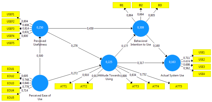
However, recently Bentler and Huang (2014), Dijkstra (2014), and Dijkstra and Henseler (2015) introduced methods that provide consistent PLS-SEM estimations. These consistent PLS (PLSc) estimations of common factor models have been designed to mimic CB-SEM (Sarstedt et al, 2016). Thereby, researchers can also use PLS-SEM to study structure (Rigdon et al., 2017). As a result, we see two developments of PLS-SEM: One direction use PLS-SEM for prediction-oriented studies and another direction uses PLS-SEM (via PLSc) to mimic CB-SEM for studies that focus on analyzing and testing the model structure.
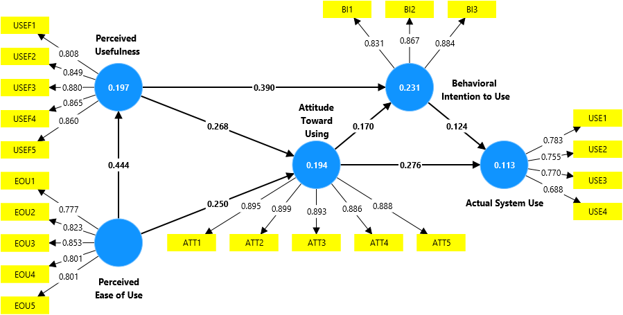
In face of these recent developments, we use an application of the well-known technology acceptance model (TAM, Davis, 1989). The model estimation uses a dataset with 1,190 responses and the SmartPLS (Ringle et al., 2022) and AMOS (Arbuckle, 2006) software (alternative structural equation modeling software solutions are, for example, EQS, LISREL, and MPLUS). You can download the TAM example, which can be imported as a project into the SmartPLS software, from the resources of this webpage.
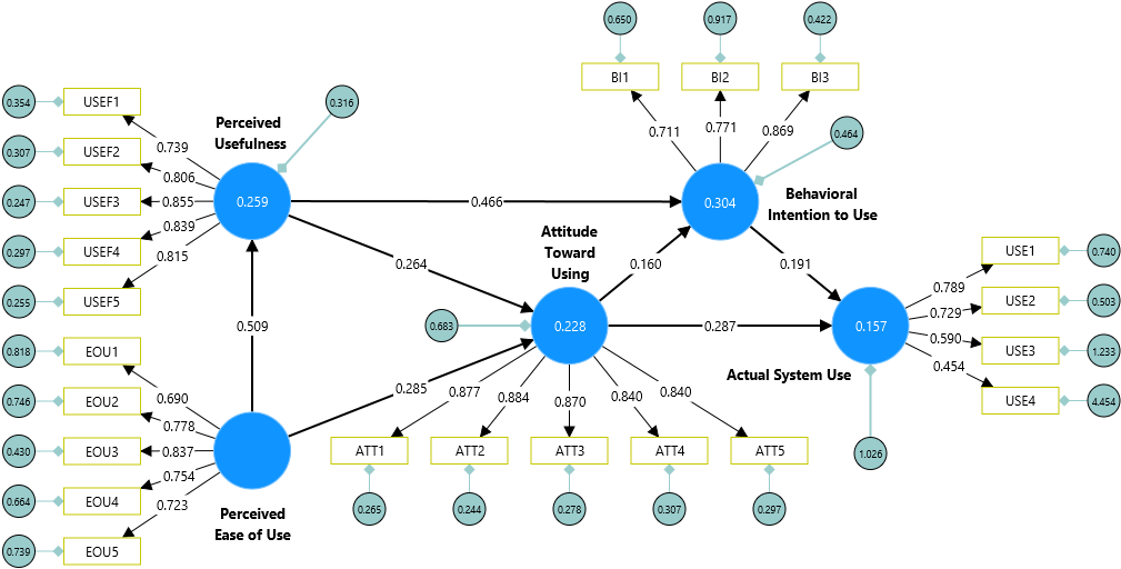
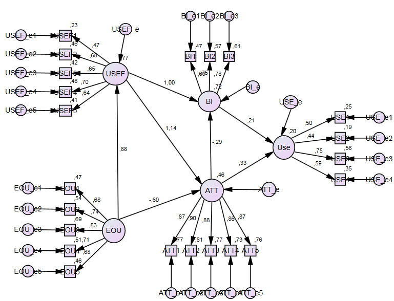
Similar to the study presented by Sartstedt et al. (2024), we used CB-SEM and PLS-SEM to estimate the model. However, we also used alternative CB-SEM estimators and added the results of the sum score regression and equal weighting. We find that the results of ML-CBSEM in AMOS and SmartPLS are identical. Interestingly, PLSc-SEM and PLS-SEM come closest to these results, and to some extent, although by a slightly larger margin, the results of sum score regression and PLS-SEM using equal weights. In contrast, it is surprising to note the large differences in results when using alternative CB-SEM estimation methods (e.g., GLS, ULS, and ADF). Therefore, the one-sided view pitting CB-SEM against PLS-SEM seems to be misleading. Rather, both model estimation methods should be considered as complementary approaches to SEM (Jöreskog & Wold, 1982). In summary, we expect the widespread use of multi-method approaches in SEM for future applications (Sarstedt et al., 2024).
Alternative model estimations
CB-SEM maximum likelihood (ML) results using AMOS (standardized coefficients)
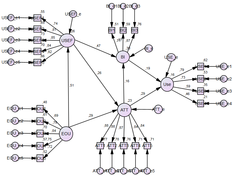
CB-SEM maximum likelihood (ML) results using SmartPLS (standardized coefficients)
PLS-SEM mimicking CB-SEM rersults via consistent PLS-SEM (PLSc-SEM) using SmartPLS
PLS-SEM results using SmartPLS

Sumscore regression results using SmartPLS
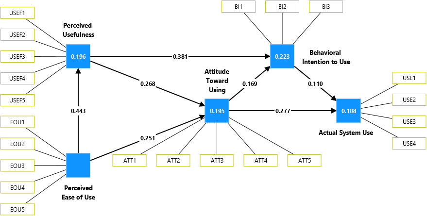
Equal weights PLS-SEM results using SmartPLS
CB-SEM generalized least squares (GLS) results using AMOS (standardized coefficients)

CB-SEM unweighted least squares (ULS) results using AMOS (standardized coefficients)

CB-SEM asymptotically distribution-free (ADF) results using AMOS (standardized coefficients)
References
- Arbuckle, J.L. 2006. "Amos (Version 7.0)." Chicago: SPSS.
- Bentler, P.M., and Huang, W. 2014. "On Components, Latent Variables, PLS and Simple Methods: Reactions to Ridgon’s Rethinking of PLS." Long Range Planning 47 (3): 138-145.
- Chin, W.W., and Newsted, P.R. 1999. "Structural Equation Modeling Analysis with Small Samples Using Partial Least Squares." In Statistical Strategies for Small Sample Research. Ed. R.H. Hoyle. Thousand Oaks: Sage, 307-341.
- Davis, F.D. 1989. "Perceived Usefulness, Perceived Ease of Use, and User Acceptance of Information Technology." MIS Quarterly 13 (3): 319-340.
- Dijkstra, T.K. 2014. "PLS' Janus Face – Response to Professor Rigdon's ‘Rethinking Partial Least Squares Modeling: In Praise of Simple Methods’." Long Range Planning 47 (3): 146-153.
- Dijkstra, T.K., and Henseler, J. 2015. "Consistent Partial Least Squares Path Modeling." MIS Quarterly 39 (2): 297-316.
- Fornell, C.G., and Bookstein, F.L. 1982. "Two Structural Equation Models: LISREL and PLS Applied to Consumer Exit-Voice Theory." Journal of Marketing Research 19 (4): 440-452.
- Hair, J.F., Ringle, C.M., and Sarstedt, M. 2011. "PLS-SEM: Indeed a Silver Bullet." Journal of Marketing Theory and Practice 19 (2): 139-151.
- Hair, J.F., Sarstedt, M., Ringle, C.M., and Mena, J.A. 2012. "An Assessment of the Use of Partial Least Squares Structural Equation Modeling in Marketing Research." Journal of the Academy of Marketing Science 40 (3): 414-433.
- Hair, J.F., Hult, G.T.M., Ringle, C.M., & Sarstedt, M. 2022. A Primer on Partial Least Squares Structural Equation Modeling (PLS-SEM), 3rd Ed., Thousand Oaks, CA: Sage.
- Hair, J.F., Sarstedt, M., Ringle, C.M., and Gudergan, S.P. 2024. Advanced Issues in Partial Least Squares Structural Equation Modeling (PLS-SEM), 2nd Ed., Thousand Oaks, CA: Sage.
- Henseler, J., Dijkstra, T.K., Sarstedt, M., Ringle, C.M., Diamantopoulos, A., Straub, D.W., Ketchen, D.J., Hair, J.F., Hult, G.T.M., and Calantone, R. J. 2014. "Common Beliefs and Reality about Partial Least Squares: Comments on Rönkkö & Evermann (2013)." Organizational Research Methods 17 (2): 182-209.
- Jöreskog, K.G., and Wold, H. 1982. "The ML and PLS Techniques For Modeling with Latent Variables: Historical and Comparative Aspects." In Systems Under Indirect Observation, Part I. Eds. H. Wold and K.G. Jöreskog. Amsterdam: North-Holland, 263-270.
- Lohmöller, J.-B. 1989. Latent Variable Path Modeling with Partial Least Squares. Heidelberg: Physica.
- Reinartz, W.J., Haenlein, M., and Henseler, J. 2009. "An Empirical Comparison of the Efficacy of Covariance-Based and Variance-Based SEM." International Journal of Research in Marketing 26 (4): 332-344.
- Rigdon, E.E. 2012. "Rethinking Partial Least Squares Path Modeling: In Praise of Simple Methods." Long Range Planning 45 (5-6): 341-358.
- Rigdon, E.E. 2014. "Rethinking Partial Least Squares Path Modeling: Breaking Chains and Forging Ahead." Long Range Planning 47 (3): 161-167.
- Rigdon/ E.E., Sarstedt, M., and Ringle, C.M. (2017). On Comparing Results from CB-SEM and PLS-SEM. Five Perspectives and Five Recommendations. Marketing ZFP, 39(3), 4-16.
- Ringle, C. M., Wende, S., and Becker, J.-M. 2024. "SmartPLS 4." Bönningstedt: SmartPLS GmbH.
- Sarstedt, M., Adler, S.J., Ringle, C.M., Cho, G., Diamantopoulos, A., Hwang, H., and Liengaard, B.D. (2024). Same Model, Same Data, But Different Outcomes: Evaluating the Impact of Method Choices in Structural Equation Modeling. Journal of Product Innovation Management.
- Sarstedt, M., Hair, J.F., Ringle, C.M., Thiele, K.O., and Gudergan, S.P. Estimation Issues with PLS and CBSEM: Where the Bias Lies!, Journal of Business Research, 69 (2016), Issue 10, pp. 3998-4010.
- Sarstedt, M., Ringle, C.M., Henseler, J., and Hair, J.F. 2014. "On the Emancipation of PLS-SEM: A Commentary on Rigdon (2012)." Long Range Planning 47 (3): 154-160.
- Wold, H. 1982. "Soft Modeling: The Basic Design and Some Extensions." In Systems Under Indirect Observations: Part II. Eds. K.G. Jöreskog and H. Wold. Amsterdam: North-Holland, 1-54.
