
Regression Bootstrapping
Regression bootstrapping is a nonparametric resampling procedure for statistical inference in linear regression. In SmartPLS (Ringle et al., 2024), the procedure repeatedly re-estimates a regression model on bootstrap samples drawn with replacement from the original data. The resulting empirical sampling distributions are used to estimate bootstrap standard errors, t values, p values, and confidence intervals for the model parameters.
Use regression bootstrapping when you want resampling-based inference for a linear regression model, for example as a robustness-oriented alternative or complement to significance tests based on analytical standard errors. For a binary dependent variable, use logistic regression, which applies maximum-likelihood estimation and has a different interpretation of coefficients and model fit (Margalina et al., 2026).
How Regression Bootstrapping Works
Suppose the original data set contains n observations. SmartPLS draws a bootstrap sample of n observations with replacement, estimates the same linear regression model, stores the requested results, and repeats this procedure many times. Because sampling is with replacement, an observation can appear more than once in a particular bootstrap sample, while another observation may not appear at all.
Across the bootstrap samples, SmartPLS obtains an empirical sampling distribution for each estimate. These distributions provide the basis for the bootstrap standard errors and confidence intervals. For a coefficient, the reported t statistic is based on the original estimate divided by its bootstrap standard error:
t = |Original sample estimate / Bootstrap standard error|
For a two-tailed test with a 5% significance level, a coefficient is statistically significant when its 95% bootstrap confidence interval does not include zero. Confidence intervals are especially informative because they show both the direction of an effect and the uncertainty surrounding its estimated magnitude.
Bootstrapping reduces reliance on a normal sampling distribution for significance testing, but it does not make the regression model assumption-free. Researchers should still evaluate the regression model itself, including potential collinearity and relevant residual diagnostics. The Regression page and the SmartPLS tutorial by Margalina et al. (2026) describe the systematic evaluation of linear regression results in more detail.
Running Regression Bootstrapping in SmartPLS
After specifying a linear regression model, select the regression bootstrapping procedure from the Calculate menu, configure the bootstrap settings, and start the calculation. For final reporting, a large number of bootstrap samples should be used. The example below uses 10,000 bootstrap samples, a two-tailed test, a 5% significance level, the percentile bootstrap, and a fixed random seed.
Bootstrapping Settings in SmartPLS
Subsamples
The Samples setting determines how many bootstrap samples SmartPLS draws. Each bootstrap sample contains the same number of observations as the original analysis sample. If case-by-case deletion is used for missing values, SmartPLS uses the corresponding reduced number of observations.
A smaller number of bootstrap samples, such as 1,000, can be useful for an initial assessment because it reduces computation time. For final results, use a large number of bootstrap samples, such as 10,000, to improve the stability of bootstrap standard errors and confidence intervals (Hair et al., 2027).
Note: Increasing the number of bootstrap samples increases computation time.
Amount of Results
The amount-of-results setting controls how much information SmartPLS stores and reports. The faster option focuses on the most important bootstrap results. The Complete (slower) option retains additional outputs and is required when you want to inspect more detailed bootstrap results, such as results at the individual bootstrap-sample level. More complete output requires additional computation time and storage.
Confidence Interval Method
The confidence interval method determines how SmartPLS converts the bootstrap distribution into a nonparametric confidence interval. SmartPLS provides three methods:
- Percentile bootstrap (default): Uses the empirical percentiles of the bootstrap distribution directly. This method is straightforward and is recommended as the default for most applications.
- Studentized bootstrap: Uses a studentized statistic that accounts for the estimated standard error within the resampling procedure. It is more computationally demanding.
- Bias-corrected and accelerated (BCa) bootstrap: Adjusts the confidence interval for bias and acceleration in the bootstrap distribution and can be useful when the distribution is asymmetric or biased.
For additional discussion of bootstrap confidence intervals, see Hair et al. (2027), Efron and Tibshirani (1993), and Davison and Hinkley (1997).
Test Type
Select a one-tailed or two-tailed significance test according to the hypothesis being tested. A directional hypothesis may justify a one-tailed test when specified a priori. Otherwise, a two-tailed test is generally appropriate.
Significance Level
The significance level determines the width of the confidence interval and the threshold used for statistical significance. For example, a two-tailed test with a significance level of 0.05 corresponds to a 95% confidence interval.
Random Number Generator
Because bootstrap samples are randomly drawn, the procedure requires a seed for the random number generator. A random seed generates different bootstrap samples when the analysis is rerun. A fixed seed reproduces the same bootstrap samples when the analysis is repeated with the same settings, which facilitates reproducibility.
For analyses reported in publications, using a fixed seed is useful when exact replication of the SmartPLS bootstrap results is desired.
Parallel Processing
Parallel processing distributes bootstrap calculations across multiple processor cores. Because the bootstrap samples can be estimated independently, parallel processing can substantially reduce computation time. It changes computation speed, not the statistical logic of the procedure.
Understanding the SmartPLS Regression Bootstrapping Results
The SmartPLS Results report separates the bootstrap output into several result groups. The most important outputs for interpreting regression bootstrapping are the following.
Unstandardized Coefficients
The unstandardized regression coefficients retain the original measurement units. They are useful when the substantive interpretation concerns the expected change in the dependent variable associated with a one-unit change in an independent variable, holding the other predictors constant (Margalina et al., 2026).
For every unstandardized coefficient, SmartPLS reports the Original sample (O), Sample mean (M), Standard deviation (STDEV), t statistic, and p value. The report also provides confidence intervals. The difference between the bootstrap sample mean and the original estimate indicates the estimated bootstrap bias.
Standardized Coefficients
Standardized coefficients express effects in standard deviation units and facilitate comparisons of the relative strength of predictors measured on different scales. SmartPLS reports the same bootstrap statistics for standardized coefficients as for unstandardized coefficients: original estimate, bootstrap mean, bootstrap standard error, t value, p value, and confidence intervals.
Statistical significance and substantive relevance should be distinguished. A small coefficient can be statistically significant, while a large coefficient can have substantial uncertainty. Therefore, interpret the coefficient magnitude together with its confidence interval rather than relying only on the p value.
R-Square, Adjusted R-Square, and VIF
The regression bootstrapping report can also provide bootstrap summaries for quality criteria such as R², adjusted R², and VIF. Bootstrap distributions for R² and adjusted R² show the sampling variability of the model's explanatory power.
For VIF, the original VIF values remain the primary diagnostic for assessing collinearity. Do not interpret a bootstrap p value for VIF as the main collinearity criterion. Instead, evaluate the VIF level against established collinearity guidelines as explained on the Regression page and in Margalina et al. (2026).
Histograms of Bootstrap Distributions
SmartPLS provides histograms for unstandardized and standardized regression coefficients. These plots visualize the empirical bootstrap distribution of an estimate and can reveal asymmetry, dispersion, or unusual tails that are not apparent from a single standard error or p value.
The gray normal curve displayed with the histogram is a reference distribution. The bootstrap procedure does not require the empirical distribution to be normal.
Example: Bootstrap Distribution of the Standardized X6 Coefficient
The following example uses the HBAT linear regression model discussed by Margalina et al. (2026). Customer satisfaction (X19) is the dependent variable, and product quality (X6), e-commerce activities/website (X7), complaint resolution (X9), product line (X11), and salesforce image (X12) are the independent variables. The regression bootstrapping run uses 10,000 bootstrap samples, percentile confidence intervals, a two-tailed test, a 5% significance level, and a fixed seed.
For the standardized coefficient of product quality (X6), the SmartPLS report gives an original estimate of 0.432, a bootstrap sample mean of 0.432, and a bootstrap standard error of 0.058. The resulting t value is 7.432 and p < 0.001. The 95% percentile bootstrap confidence interval ranges from 0.321 to 0.551, while the additional bias-corrected interval reported by SmartPLS ranges from 0.324 to 0.554. Both intervals exclude zero, providing clear evidence of a positive relationship between product quality and customer satisfaction in this model.
The bootstrap mean is almost identical to the original standardized coefficient, indicating negligible bootstrap bias for this estimate. The histogram is centered around approximately 0.43 and is reasonably symmetric, which is consistent with the numerical bootstrap results.
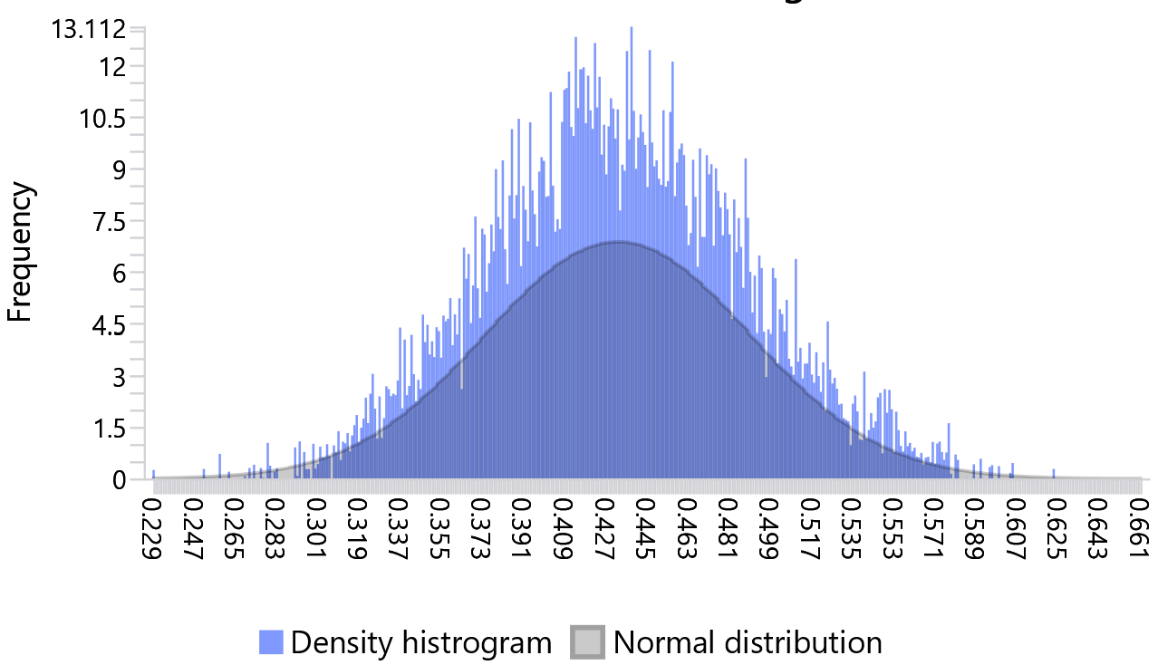
Figure: Bootstrap frequency/density histogram of the standardized regression coefficient for X6 (product quality). The blue bars show the empirical bootstrap distribution, and the gray curve provides a normal-distribution reference.
The same Results report shows R² = 0.791 for the model. Across the 10,000 bootstrap samples, the mean R² is 0.800, with a 95% percentile confidence interval from 0.724 to 0.863. These results illustrate how regression bootstrapping can be used not only to assess coefficient inference but also to quantify sampling variability in model-level results.
Regression Bootstrapping Versus Linear and Logistic Regression Inference
The Regression algorithm estimates linear regression coefficients and provides the standard model evaluation results, including analytical significance tests and diagnostic criteria. Regression bootstrapping re-estimates the same linear regression model across many resampled data sets to obtain resampling-based standard errors, p values, confidence intervals, and distributions.
Logistic Regression is different because the dependent variable is binary and the model is estimated by maximum likelihood. Logistic regression coefficients represent changes in log-odds rather than changes in a metric dependent variable, and SmartPLS reports likelihood-based model fit and Wald tests (Margalina et al., 2026). Therefore, the interpretation of logistic regression should follow the dedicated logistic regression guidance rather than the linear regression bootstrapping procedure described on this page.
Frequently Asked Questions
What does regression bootstrapping test?
Regression bootstrapping evaluates the sampling uncertainty of linear regression estimates by repeatedly resampling the observations with replacement and re-estimating the model. SmartPLS uses the resulting empirical distributions to calculate bootstrap standard errors, t values, p values, and confidence intervals.
How many bootstrap samples should I use?
For an initial check, about 1,000 bootstrap samples can be sufficient and faster to compute. For final results, use a large number such as 10,000 to obtain more stable estimates of bootstrap standard errors and confidence intervals.
Which confidence interval method should I choose?
The percentile bootstrap is the SmartPLS default and is recommended for most applications. The BCa bootstrap is an alternative when bias or asymmetry in the bootstrap distribution is a concern. The studentized bootstrap provides another alternative but is computationally more demanding.
How do I determine whether a regression coefficient is significant?
For a two-tailed test at the 5% significance level, inspect the 95% bootstrap confidence interval. If the interval does not include zero, the coefficient is statistically significant at the 5% level. SmartPLS also reports the corresponding t value and p value.
Should I report unstandardized or standardized coefficients?
Report unstandardized coefficients when interpretation in the original measurement units is important. Standardized coefficients are useful for comparing the relative strength of predictors. In many applications, reporting both provides the most complete interpretation.
Does bootstrapping eliminate the need to check regression assumptions?
No. Bootstrapping changes how sampling uncertainty and statistical inference are estimated, but it does not correct a misspecified regression model, problematic collinearity, dependent observations, endogeneity, or other design and model-specification problems. Continue to assess the regression model and its diagnostics.
Why should I use a fixed seed?
A fixed seed makes the random resampling sequence reproducible. If the same data, model, number of bootstrap samples, and other settings are used, rerunning the analysis produces the same bootstrap results.
Does parallel processing change the results?
No. Parallel processing only distributes the bootstrap calculations across processor cores to reduce computation time; it does not change the resampling logic or the interpretation of the results.
Related SmartPLS Methods
References
- Davison, A. C., & Hinkley, D. V. (1997). Bootstrap methods and their application. Cambridge University Press.
- Efron, B., & Tibshirani, R. J. (1993). An introduction to the bootstrap. Chapman & Hall.
- Hair, J. F., Hult, G. T. M., Ringle, C. M., & Sarstedt, M. (2027). A Primer on Partial Least Squares Structural Equation Modeling (PLS-SEM) (4 ed.). Sage.
- Margalina, V.-M., Kreienbaum, C., Hair, J. F., Becker, J.-M., & Ringle, C. M. (2026). Multiple linear and logistic regression analysis: a SmartPLS 4 software tutorial. Journal of Marketing Analytics, 14, 709–726.
- Ringle, C. M., Wende, S., & Becker, J.-M. (2024). SmartPLS 4. In SmartPLS. https://www.smartpls.com/
- More literature ...
Cite correctly
Please always cite the use of SmartPLS!
Ringle, Christian M., Wende, Sven, & Becker, Jan-Michael. (2024). SmartPLS 4. Bönningstedt: SmartPLS. Retrieved from https://www.smartpls.com
